AI Class: Tile Puzzle Heuristics

In an earlier post, I presented some code for solving tile puzzles using A* search. In the lectures, Peter Norvig talked about two different heuristics for these puzzles, one simply counting the number of misplaced tiles and the other giving the total Manhattan distance of all misplaced tiles to their correct positions. It’s interesting to find out how much of a difference using these heuristics really makes.

State space size

First question: how many states do these problems actually have? For an $n \times n$ puzzle, we generate an arbitrary state by placing $n^2-1$ tiles into $n^2$ positions, which means that there are, on the face of it, $(n^2)!$ possible states. However, states have a kind of parity, which means that the state space is partitioned into two mutually exclusive halves. Using only legal moves of the blank position in the puzzle, there are only $(n^2)!/2$ positions accessible from the “perfect” initial state.

For a $3 \times 3$ puzzle, $(n^2)!/2 = 181,440$ and for a $4 \times 4$ puzzle, $(n^2)!/2 = 10,461,394,944,000 \approx 10^{13}$, which is a big number. In the $3 \times 3$ case, we can just about imagine exploring a reasonable fraction of the full state space to find the solution. For the $4 \times 4$ case, we have no hope of exploring more than a tiny fraction of the state space. The number of states that any particular algorithm needs to expand to find a solution will obviously depend on the starting state: some states are only a move or two away from the goal state, so solutions are easy to find, while others are “a long way away” in state space (whatever the metric is that we might define).

What we do

Here’s what we do: we generate a whole bunch of random start states, each a given number of “scrambling” moves from the perfect state. We try to solve each of those using uniform cost search (Heuristic 0, i.e. a heuristic of zero for all states), the misplaced tile count heuristic (which we’ll call Heuristic 1) and the total Manhattan distance heuristic (Heuristic 2). We record the number of search tree nodes that need to be explored to find a solution for each case (I set a ceiling of 10000 nodes just so I can finish a reasonable number of computations on my aging laptop). What we end up with is a set of tuples $(n, s, h, c)$, where $n$ is the problem size (3 or 4), $s$ is the number of “scrambling” moves (between 10 and 100), $h$ is the heuristic (0, 1 or 2) and $c$ is the cost, i.e. the number of nodes expanded. We can then look at plots of $c$ for different combinations of $n$, $s$ and $h$. Below, I’ll show results from all the heuristics and “scrambling distance” together, with one plot for each problem size.

Results

Let’s look at the $3 \times 3$ case first. This plot shows the number of nodes expanded for a range of scrambling moves for all three heuristics. For each heuristic and each scrambling move count, the box-and-whisker plots show the results of 1000 runs from random initial states:

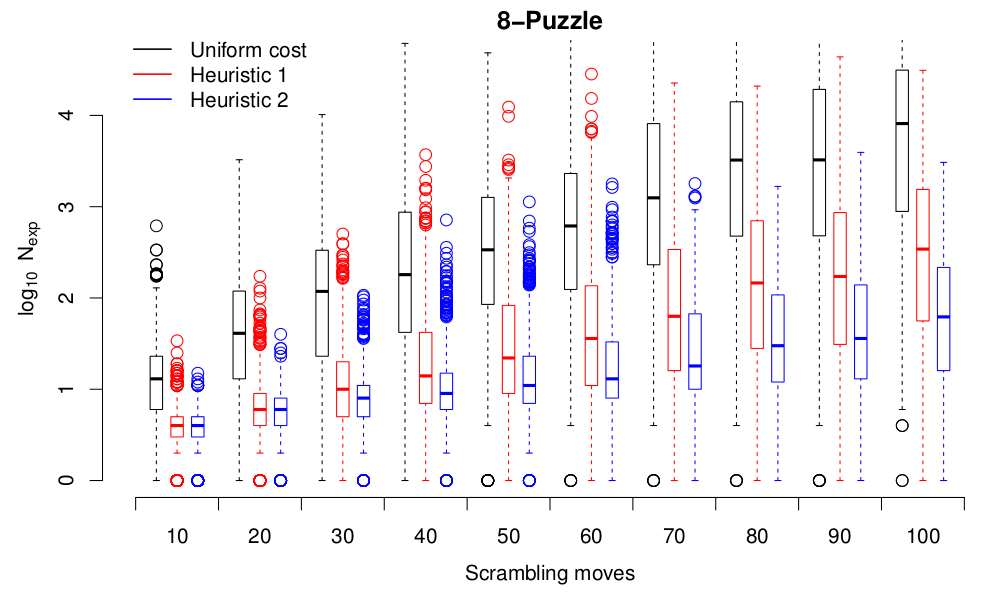
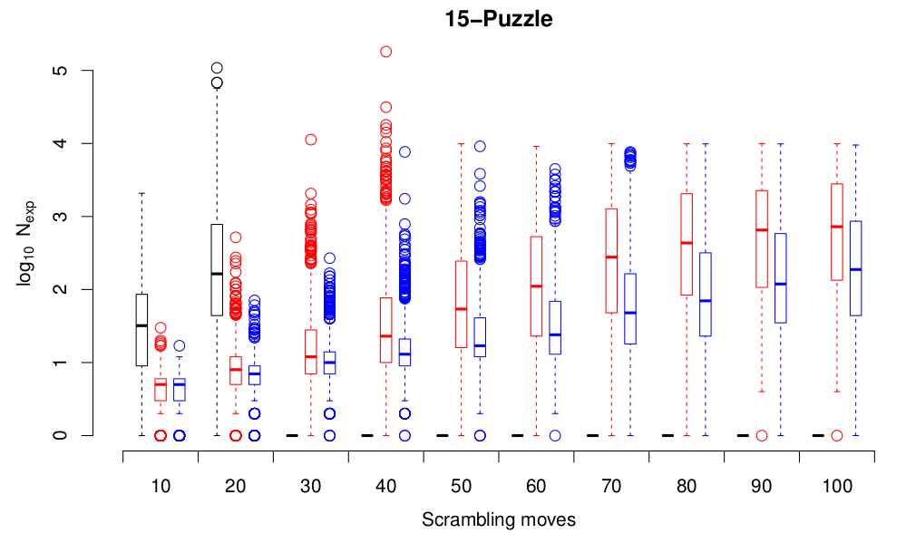
Note the log scale for the number of nodes expanded! Using heuristics really does seem to make a difference. And the heuristic that we choose also makes quite a difference–Heuristic 2 is appreciably better than Heuristic 1. The story is the same for the $4 \times 4$ case. Here, I wasn’t patient enough to wait for all the uniform cost search results, since they take a long time. I’ve also limited the number of nodes expanded to 10,000, so things finish up in a sensible timeframe.

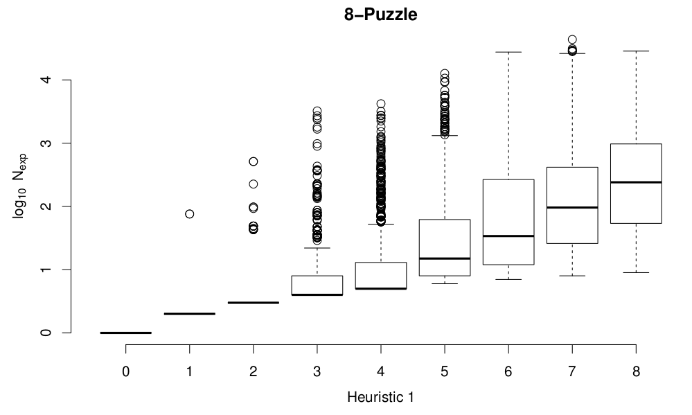
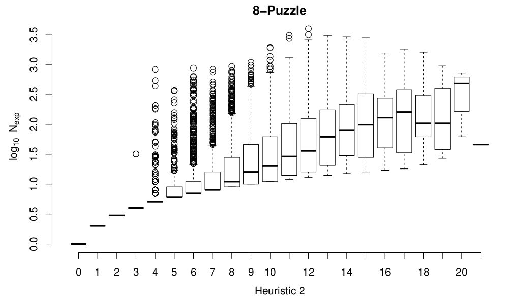
One thing that’s clear on these plots is that there’s a very big spread in the cost of starting from different states the same “scrambling distance” from the goal state. That’s expected: consider two states at a “scrambling distance” of 3 from the initial state, one of which consists of moving the blank left, right, left and the other left, up, left. The first state has two moves that are inverses of one another, so the resulting state is only one move from the goal state, while the second one requires three moves to get back to the goal state. So perhaps “scrambling distance” isn’t the best metric to use on the state space. What other metrics could we use? Well, we have two ready-made, in the form of the heuristics. As well as perhaps giving us a better view of the performance of the heuristics in terms of actually helping to solve the puzzles, plotting the node expansion costs as a function of the heuristic values will also show us how well the heuristics do at measuring how hard it is to solve from a given initial state. Here are results for the 8-puzzle:

and the for 15-puzzle:

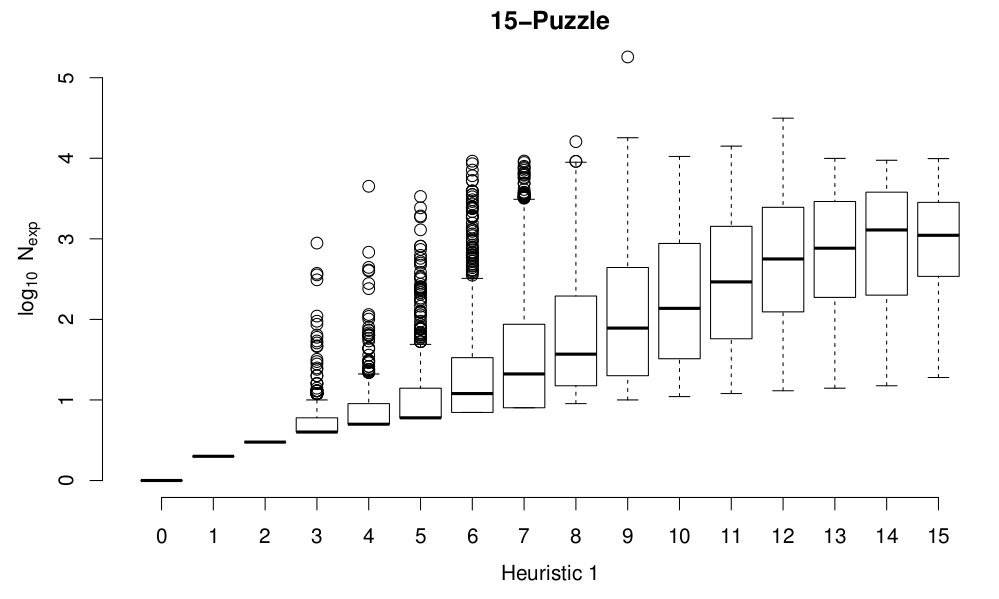
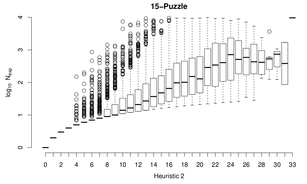
Although the spread at the top range of the costs is artificially compressed because I terminate any solves that expand more than 10,000 nodes, it seems pretty clear from these plots that both heuristics do a reasonable job of approximating the likely solution cost for a given initial configuration of the board. Heuristic 2 divides states up more finely than Heuristic 1, and is definitely a more accurate heuristic, in terms of being less optimistic while still admissible.

Conclusions

The conclusions are pretty clear: A* search with a good heuristic works much better on problems with realistically sized search spaces than a simple uniform cost search. We end up needing to explore a far smaller portion of search space to find solutions. The key thing here is that A* search is guaranteed to find the optimal solution, provided that the heuristic we use is optimistic. There is a partial order on admissible heuristics for a given problem, where we can produce heuristics that are more and more accurate, i.e. less and less optimistic, and thus produce a better and better assessment of how far a particular state is from the goal.

A couple of points about this example. First, we’re solving these tile puzzles in kind of a dumb way. We could introduce a much more structured way of thinking about permissible moves (we can think of “circulating” sets of tiles as a single move, for instance, which immediately allows us to jump around in state space in more interesting ways). Second, A* search runs out of memory sometimes. And in this problem, it runs out of memory unpredictably: given two initial states, both generated from the goal state by 50 scrambling moves, one may take only 500 node expansions to solve, the other may take more than 10,000. Given unlimited memory, A* search will find the solution eventually, but we keep hold of a lot of “junk” states in the search space that are really of no use at all. There are more sophisticated algorithms for this sort of search that can run in limited memory, by discarding some of those redundant states.

Anyway, the take home lesson is that heuristics are important for search!