Haskell FFT 4: A Simple Application

[The code from this article is available as a Gist.]

Before we go on to look at how to deal with arbitrary input vector lengths (i.e. not just powers of two), let’s try a simple application of the powers-of-two FFT from the last article.

We’re going to do some simple frquency-domain filtering of audio data. We’ll start with reading WAV files. We can use the Haskell WAVE package to do this–it provides functions to read and write WAV files and has data structures for representing the WAV file header information and samples.

We’ll use a sort of sliding window FFT to process the samples from each channel in the WAV file. Here’s how this works:

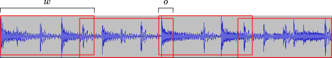
We split the audio samples up into fixed-length “windows” (each $w$ samples long) with adjacent windows overlapping by $o$ samples. We select $w$ to be a power of 2 so that we can use our power-of-two FFT algorithm from the last section. We calculate the FFT of each window, and apply a filter to the spectral components (just by multiplying each spectral component by a frequency-dependent number). Then we do an inverse FFT, cut off the overlap regions and reassemble the modified windows to give a filtered signal.

I’m not going to talk much about the details of audio filtering here. Suffice it to say that what we’re doing isn’t all that clever and is mostly just for a little demonstration–we’ll definitely be able to change the sound of our audio, but this isn’t a particularly good approach to denoising speech. There are far better approaches to that, and I may talk about them at some point in the future.

Anyway, let’s look at some code:

-- A filter specifies a window size, a window overlap (both in terms
-- of numbers of samples) and a filter function (which should be a
-- window size length vector).
data Filter = Filter { fWindowSize :: Int
                     , fWindowOverlap :: Int
                     , fFilterFunc :: Vector (Complex Double) }

-- Helper for building filter functions.
build :: [(Int, Int)] -> Vector (Complex Double)
build segs = map realToFrac $ concat $ P.map (\(n, v) -> replicate n v) segs

-- Smooth filter function.
smooth :: Vector (Complex Double)
smooth = map realToFrac $ generate 1024 $ \i ->
  cos (2 * pi * fromIntegral i / 1023)

-- Some filters: at a sampling rate of 44100 Hz, 1024 samples is about
-- 0.02 seconds.
filt_noop, filt_hard, filt_hard_olap :: Filter
filt_smooth, filt_smooth_olap :: Filter
filt_noop = Filter 1024 0 (build [(1024,1)])
filt_hard = Filter 1024 0 (build [(128,1), (768,0), (128,1)])
filt_hard_olap = Filter 1024 256 (build [(128,1), (768,0), (128,1)])
filt_smooth = Filter 1024 0  smooth
filt_smooth_olap = Filter 1024 256 smooth
filters :: [Filter]
filters = [filt_noop, filt_hard, filt_hard_olap, filt_smooth, filt_smooth_olap]

First we define a very simple data structure for holding the information about a filter and we define some filters. The filtering function is defined as a vector of complex numbers (which must be the same length as the window size we specify), and we apply it just by multiplying into the spectra element-by-element. One thing we’re not bothering with here is power equalisation–if we use a filtering function that radically alters the overall magnitudes of the audio samples, we’ll end up with something that sounds much louder or softer than the original. It’s better to stick with filtering functions $f$ for which $\int_{-\infty}^\infty |f(x)|^2 \, dx = 1$. We’ll gloss over this detail. (We’re also not going to talk about windowing functions or anything else filtering-related. This is an example where we’re going to take almost the dumbest approach possible just to have a play.

Then we have a simple driver to read our WAV file, apply the filter (using the runFilter function) and write the result back to a new WAV file:

-- Main processing driver.
doit :: Filter -> String -> String -> IO ()
doit filt@(Filter win o _) fin fout = do
  -- Read WAV file.
  w <- getWAVEFile fin

  -- Powers of two only.
  let h = waveHeader w
      Just nsamp = waveFrames h
      nwins = (nsamp + o) `div` (win - o)
      nsampout = (win - o) * nwins

  -- Convert all channels to Vector (Complex Double) and extract
  -- individual channels as vectors.
  let d = fromList $ P.map (map sampleToDouble . fromList) $
          P.take (nsampout + o) $ waveSamples w
      chs = map (\i -> map (!i) d) $ enumFromN 0 (waveNumChannels h)

  -- Run filter.
  let chout = map (runFilter filt) chs

  -- Convert data back to frames and write out.
  let dout = map (\i -> map (!i) chout) $ enumFromN 0 nsampout
      sampout = toList $ map (toList . map doubleToSample) dout
      wave = WAVE ((waveHeader w) { waveFrames = Just nsampout }) sampout
  putWAVEFile fout wave

The only slight annoyance here is flipping back and forth between the WAV files “frame”-based view, which bundles all the samples at one time point for all channels together, and a channel-based view, where we get all the samples for a channel as a single vector that we can manipulate. We also deal with making sure that the signal we pass to the filter fits the window and overlap sizes we’re using.

Finally, we have the audio filtering pipeline itself:

-- Handy pipeline combinator.
(=>=) :: (a -> b) -> (b -> c) -> a -> c
(=>=) = flip (.)

-- Apply a filter to a channel.
runFilter :: Filter -> Vector Double -> Vector Double
runFilter (Filter w o ffn) din = proc ss
  where
    -- Data to Complex Double for our complex-to-complex FFT.
    cdin = map realToFrac din

    -- Window start positions.
    ss = enumFromStepN 0 (w - o) ((length din + o) `div` (w - o))

    -- Processing pipeline.
    proc =     map (\s -> slice s w cdin)      -- Extract windows.
           =>= map fft
           =>= map (zipWith (*) ffn)           -- Filter.
           =>= map ifft
           =>= map (slice (o `div` 2) (w - o)) -- Slice off overlaps.
           =>= toList =>= concat               -- Concatenate windows.
           =>= map realPart                    -- Convert back to real data.

We define a handy sequencing operator which is just normal function composition with the arguments reversed (oddly enough, this doesn’t seem to have a standard name in Haskell), so we can just string operations together in something that looks like a signal processing pipeline. We slice up the data into windows, Fourier transform, apply the filtering function, inverse Fourier transform, cut off the window overlaps, concatenate everything back together and convert back to real values and we’re done.

This is all wrapped up into a little standalone program that we can run from the command line giving input and output WAV file names, along with an index into the filters list to select a filter to apply. So, what can we do with this? I recorded a few seconds of speech using no care at all and the crappiest microphone I could find, producing a WAV file with lots of noise. Let’s apply a series of different filters to it and see what we get. In all cases, we take a window size of 1024 samples (about 0.02 s at a sample rate of 44,100 Hz). We use a window-to-window overlap of either zero or 256 samples (i.e. a quarter of the window length at each end is overlapped with the adjacent windows), and we either use a “hard” filter which cuts out the middle half of the spectral elements (corresponding to zeroing out spectral components for frequencies above about 11 kHz) or a “smooth” cosine-shaped filter (which is one at zero frequency and falls to zero at the Nyquist frequency).

The following links go to WAV files:

• Original signal–very noisy, sounds like it might have been recorded on one of Thomas Edison’s old wax cylinder rigs.

• No overlap, hard filter–slightly less noisy, but it sounds like I’m in a bucket and you can hear a “clicking” artefact from the lack of window overlap.

• Overlap, hard filter–less noise, no clicking, still a little bit “buckety”.

• No overlap, smooth filter–same clicking artefact as in the “hard” filter case with no overlap.

• Overlap, soft filter–less noise, no clicking, not very buckety: definitely the best result.

There’s obviously relatively little merit to this in terms of making the sound sound nicer, but it shows how easy it is to fiddle with this kind of audio processing–the “filtering” function we’ve been using is a complex vector, so we could do all sorts of phase shifting things with it as well as modifying the amplitudes of the spectral components.

Anyway, I thought a post with no equations in it at all might be a nice break. In the next article, there will be quite a lot of equations and a fair bit head-scratching as we extend the “toy algebra” system to help understand the mixed-radix FFT for arbitrary vector lengths.