Non-diffusive atmospheric flow #7: PCA for spatio-temporal data
Although the basics of the “project onto eigenvectors of the covariance matrix” prescription do hold just the same in the case of spatio-temporal data as in the simple two-dimensional example we looked at in the earlier article, there are a number of things we need to think about when we come to look at PCA for spatio-temporal data. Specifically, we need to think bout data organisation, the interpretation of the output of the PCA calculation, and the interpretation of PCA as a change of basis in a spatio-temporal setting. Let’s start by looking at data organisation.
The anomaly data we want to analyse has 66 × 151 = 9966 days of data, each of which has 72 × 15 = 1080 spatial points. In our earlier two-dimensional PCA example, we performed PCA on a collection of two-dimensional data points. For the data, it’s pretty clear that the “collection of points” covers the time steps, and each “data point” is a 72 × 15 grid of values. We can think of each of those grids as a 1080-dimensional vector, just by flattening all the grid values into a single row, giving us a sequence of “data points” as vectors in that we can treat in the same kind of way as we did the two-dimensional data points in the earlier example. Our input data thus ends up being a set of 9966 1080-dimensional vectors, instead of 500 two-dimensional vectors (as for the mussel data). If we do PCA on this collection of 1080-dimensional vectors, the PCA eigenvectors will have the same shape as the input data vectors, so we can interpret them as spatial patterns, just by inverting the flattening we did to get from spatial maps of to vectors — as long as we interpret each entry in the eigenvectors as the same spatial point as the corresponding entry in the input data vectors, everything works seamlessly. The transformation goes like this:
pattern → vector → PCA → eigenvector → eigenpattern
So we have an interpretation of the PCA eigenvectors (which we’ll henceforth call “PCA eigenpatterns” to emphasise that they’re spatial patterns of variability) in this spatio-temporal data case. What about the PCA eigenvalues? These have exactly the same interpretation as in the two-dimensional case: they measure the variance “explained” by each of the PCA eigenpatterns. And finally, the PCA projected components tell us how much of each PCA eigenpattern is present in each of the input data vectors. Since our input data has one spatial grid per time step, the projections give us one time series for each of the PCA eigenvectors, i.e. one time series of PCA projected components per spatial point in the input. (In one way, it’s kind of obvious that we need this number of values to reproduce the input data perfectly — I’ll say a little more about this when we think about what “basis” means in this setting.)
The PCA calculation works just the same as it did for the two-dimensional case: starting with our 1080-dimensional data, we centre the data, calculate the covariance matrix (which in this case is a 1080 × 1080 matrix, the diagonal entries of which measure the variances at each spatial point and the off-diagonal entries of which measure the covariances between each pair of spatial points), perform an eigendecomposition of the covariance matrix, then project each of the input data points onto each of the eigenvectors of the covariance matrix.
We’ve talked about PCA as being nothing more than a change of basis, in the two-dimensional case from the “normal” Euclidean basis (with unit basis vectors pointing along the x- and y-coordinate axes) to another orthnormal basis whose basis vectors are the PCA eigenvectors. How does this work in the spatio-temporal setting? This is probably the point that confuses most people in going from the simple two-dimensional example to the N-dimensional spatio-temporal case, so I’m going to labour the point a bit to make things as clear as possible.
First, what’s the “normal” basis here? Each time step of our input data specifies a value at each point in space — we have one number in our data vector for each point in our grid. In the two-dimensional case, we had one number for each of the mussel shell measurements we took (length and width). For the data, the 1080 data values are the values measured at each of the spatial points. In the mussel shell case, the basis vectors pointed in the x-axis direction (for shell length) and the y-axis direction (for the shell width). For the case, we somehow need basis vectors that point in each of the “grid point directions”, one for each of the 1080 grid points. What do these look like? Imagine a spatial grid of the same shape (i.e. 72 × 15) as the data, where all the grid values are zero, except for one point, which has a grid value of one. That is a basis vector pointing in the “direction” of the grid point with the non-zero data value. We’re going to call this the “grid” basis for brevity. We can represent the value at any spatial point (i, j) as
where is zero unless k = 15(i - 1) + j, in which case it’s one (i.e. it’s exactly the basis element we just described, where we’re numbering the basis elements in row-major order) and is a “component” in the expansion of the field using this grid basis. Now obviously here, because of the basis we’re using, we can see immediately that , but this expansion holds for any orthnormal basis, so we can transform to a basis where the basis vectors are the PCA eigenvectors, just as for the two-dimensional case. If we call these eigenvectors , then
where the are the components in the PCA eigenvector basis. Now though, the aren’t just the “zero everywhere except at one point” grid basis vectors, but they can have non-zero values anywhere.
Compare this to the case for the two-dimensional example, where we started with data in a basis that had seperate measurements for shell length and shell width, then transformed to the PCA basis where the length and width measurements were “mixed up” into a sort of “size” measurement and a sort of “aspect ratio” measurement. The same thing is happening here: instead of looking at the data in terms of the variations at individual grid points (which is what we see in the grid basis), we’re going to be able to look at variations in terms of coherent spatial patterns that span many grid points. And because of the way that PCA works, those patterns are the “most important”, in the sense that they are the orthogonal (which in this case means uncorrelated) patterns that explain the most of the total variance in the data.
As I’ve already mentioned, I’m going to try to be consistent in terms of the terminology I use: I’m only ever going to talk about “PCA eigenvalues”, “PCA eigenpatterns”, and “PCA projected components” (or “PCA projected component time series”). Given the number of discussions I’ve been involved in in the past where people have been talking past each other just because one person means one thing by “principal component” and the other means something else, I’d much rather pay the price of a little verbosity to avoid that kind of confusion.
PCA calculation
The PCA calculation for the data can be done quite easily in Haskell. We’ll show in this section how it’s done, and we’ll use the code to address a couple of remaining issues with how spatio-temporal PCA works (specifically, area scaling for data in latitude/longitude coordinates and the relative scaling of PCA eigenpatterns and projected components).
There are three main steps to the PCA calculation: first we need to centre our data and calculate the covariance matrix, then we need to do the eigendecomposition of the covariance matrix, and finally we need to project our original data onto the PCA eigenvectors. We need to think a little about the data volumes involved in these steps. Our data has 1080 spatial points, so the covariance matrix will be a 1080 × 1080 matrix, i.e. it will have 1,166,400 entries. This isn’t really a problem, and performing an eigendecomposition of a matrix of this size is pretty quick. What can be more of a problem is the size of the input data itself — although we only have 1080 spatial points, we could in principle have a large number of time samples, enough that we might not want to read the whole of the data set into memory at once for the covariance matrix calculation. We’re going to demonstrate two approaches here: in the first “online” calculation, we’ll just read all the data at once and assume that we have enough memory; in the second “offline” approach, we’ll only ever read a single time step of data at a time into memory. Note that in both cases, we’re going to calculate the full covariance matrix in memory and do a direct eigendecomposition using SVD. There are offline approaches for calculating the covariance and there are iterative methods that allow you to calculate some eigenvectors of a matrix without doing a full eigendecomposition, but we’re not going to worry about that here.
Online PCA calculation
As usual, the code is in a Gist.
For the online calculation, the PCA calculation itself is identical to our two-dimensional test case and we reuse the pca function from the earlier post. The only thing we need to do is to read the data in as a matrix to pass to the pca function. In fact, there is one extra thing we need to do before passing the anomaly data to the pca function. Because the data is sampled on a regular latitude/longitude grid, grid points near the North pole correspond to much smaller areas of the earth than grid points closer to the equator. In order to compensate for this, we scale the anomaly data values by the square root of the cosine of the latitude — this leads to covariance matrix values that scale as the cosine of the latitude, which gives the correct area weighting. The listing below shows how we do this. First we read the NetCDF data then we use the hmatrix build function to construct a suitably scaled data matrix:
Right z500short <- get innc z500var :: RepaRet3 CShort

  -- Convert anomaly data to a matrix of floating point values,
  -- scaling by square root of cos of latitude.
  let latscale = SV.map (\lt -> realToFrac $ sqrt $ cos (lt / 180.0 * pi)) lat
      z500 = build (ntime, nspace)
             (\t s -> let it = truncate t :: Int
                          is = truncate s :: Int
                          (ilat, ilon) = divMod is nlon
                          i = Repa.Z Repa.:. it Repa.:. ilat Repa.:. ilon
                        in (latscale ! ilat) *
                           (fromIntegral $ z500short Repa.! i)) :: Matrix Double
Once we have the scaled anomaly data in a matrix, we call the pca function, which does both the covariance matrix calculation and the PCA eigendecomposition and projection, then write the results to a NetCDF file. We end up with a NetCDF file containing 1080 PCA eigenpatterns, each with 72 × 15 data points on our latitude/longitude grid and PCA projected component time series each with 9966 time steps.
One very important thing to note here is the relative scaling of the PCA eigenpatterns and the PCA projected component time series. In the two-dimensional mussel shell example, there was no confusion about the fact that the PCA eigenvectors as we presented them were unit vectors, and the PCA projected components had the units of length measured along those unit vectors. Here, in the spatio-temporal case, there is much potential for confusion (and the range of conventions in the climate science literature doesn’t do anything to help alleviate that confusion). To make things very clear: here, the PCA eigenvectors are still unit vectors and the PCA projected component time series have the units of !
The reason for the potential confusion is that people quite reasonably like to draw maps of the PCA eigenpatterns, but they also like to think of these maps as being spatial patterns of variation, not just as basis vectors. This opens the door to all sorts of more or less reputable approaches to scaling the PCA eigenpatterns and projected components. One well-known book on statistical analysis in climate research suggests that people should scale their PCA eigenpatterns by the standard deviation of the corresponding PCA projected component time series and the values of the PCA projected component time series should be divided by their standard deviation. The result of this is that the maps of the PCA eigenpatterns look like maps and all of the PCA projected component time series have standard deviation of one. People then talk about the PCA eigenpatterns as showing a “typical ± 1 SD” event.
Here, we’re going to deal with this issue by continuing to be very explicit about what we’re doing. In all cases, our PCA eigenpatterns will be unit vectors, i.e. the things we get back from the pca function, without any scaling. That means that the units in our data live on the PCA projected component time series, not on the PCA eigenpatterns. When we want to look at a map of a PCA eigenpattern in a way that makes it look like a “typical” deviation from the mean (which is a useful thing to do), we will say something like “This plot shows the first PCA eigenpattern scaled by the standard deviation of the first PCA projected component time series.” Just to be extra explicit!
Offline PCA calculation
The “online” PCA calculation didn’t require any extra work, apart from some type conversions and the area scaling we had to do. But what if we have too much data to read everything into memory in one go? Here, I’ll show you how to do a sort of “offline” PCA calculation. By “offline”, I mean an approach that only ever reads a single time step of data from the input at a time, and only ever writes a single time step of the PCA projected component time series to the output at a time.
Because we’re going to be interleaving calculation and I/O, we’re going to need to make our PCA function monadic. Here’s the main offline PCA function:
pcaM :: Int -> (Int -> IO V) -> (Int -> V -> IO ()) -> IO (V, M)
pcaM nrow readrow writeproj = do
  (mean, cov) <- meanCovM nrow readrow
  let (_, evals, evecCols) = svd cov
      evecs = fromRows $ map evecSigns $ toColumns evecCols
      evecSigns ev = let maxelidx = maxIndex $ cmap abs ev
                         sign = signum (ev ! maxelidx)
                     in cmap (sign *) ev
      varexp = scale (1.0 / sumElements evals) evals
      project x = evecs #> (x - mean)
  forM_ [0..nrow-1] $ \r -> readrow r >>= writeproj r . project
  return (varexp, evecs)
It makes use of a couple of convenience type synonyms:
type V = Vector Double
type M = Matrix Double
The pcaM function takes as arguments the number of data rows to process (in our case, the number of time steps), an IO action to read a single row of data (given the zero-based row index), and an IO action to write a single row of PCA projected component time series data. As with the “normal” pca function, the pcaM function returns the PCA eigenvalues and PCA eigenvectors as its result.
Most of the pcaM function is the same as the pca function. There are only two real differences. First, the calculation of the mean and covariance of the data uses the meanCovM function that we’ll look at in a moment. Second, the writing of the PCA projected component time series output is done by a monadic loop that uses the IO actions passed to pcaM to alternately read, project and write out rows of data (the pca function just returned the PCA projected component time series to its caller in one go).
Most of the real differences to the pca function lie in the calculation of the mean and covariance of the input data:
meanCovM :: Int -> (Int -> IO V) -> IO (V, M)
meanCovM nrow readrow = do
  -- Accumulate values for mean calculation.
  refrow <- readrow 0
  let maddone acc i = do
        row <- readrow i
        return $! acc + row
  mtotal <- foldM maddone refrow [1..nrow-1]

  -- Calculate sample mean.
  let mean = scale (1.0 / fromIntegral nrow) mtotal

  -- Accumulate differences from mean for covariance calculation.
  let refdiff = refrow - mean
      caddone acc i = do
        row <- readrow i
        let diff = row - mean
        return $! acc + (diff `outer` diff)
  ctotal <- foldM caddone (refdiff `outer` refdiff) [1..nrow-1]

  -- Calculate sample covariance.
  let cov = scale (1.0 / fromIntegral (nrow - 1)) ctotal

  return (mean, cov)
Since we don’t want to read more than a single row of input data at a time, we need to explicitly accumulate data for the mean and covariance calculations. That means making two passes over the input data file, reading a row at a time — the maddone and caddone helper functions accumulate a single row of data for the mean and covariance calculations. The accumulator for the mean is pretty obvious, but that for the covariance probably deserves a bit of comment. It uses the hmatrix outer function to calculate (where is the ith data row (as a column vector) and is the data mean), which is the appropriate contribution to the covariance matrix for each individual data row.
Overall, the offline PCA calculation makes three passes over the input data file (one for the mean, one for the covariance, one to project the input data onto the PCA eigenvectors), reading a single data row at a time. That makes it pretty slow, certainly far slower than the online calculation, which reads all of the data into memory in one go, then does all the mean, covariance and projection calculations in memory, and finally writes out the PCA projected components in one go. However, if you have enough data that you can’t do an online calculation, this is the way to go. You can obviously imagine ways to make this more efficient, probably by reading batches of data rows at a time. You’d still need to do three passes over the data, but batching the reads would make things a bit quicker.
Visualising the PCA results
There are three things we can look at that come out of the PCA analysis of the anomaly data: the PCA eigenvalues (best expressed as “fraction of variance explained”), the PCA eigenpatterns and the PCA projected component time series.
First, let’s look at the eigenvalues. This plot shows the fraction of variance explained for the first 100 PCA eigenvalues of the anomaly data, both individually (blue) and cumulatively (orange):

The eigenvalues are ordered in decreasing order of magnitude in what’s usually called a “scree plot”. The reason for the name is pretty obvious, since the eigenvalues fall off quickly in magnitude giving the graph the look of cliff face with a talus slope at its foot. We often look for a “knee” in a plot like this to get some idea of how many PCA eigenpatterns we need to consider to capture a good fraction of the total variance in the data we’re looking at. Here we can see that just ten of the PCA eigenpatterns explain about half of the total variance in the anomaly data (which is a set of 1080-dimensional vectors, remember). However, there’s not all that much of a “knee” in the scree plot here, which is pretty typical for climate and meteorological data — we often see a gradual fall-off in PCA eigenvalue magnitude rather than a discrete set of larger magnitude eigenvalues that we can identify as “the important ones”.
We can get some idea of what’s going on with this gradual fall-off by looking at the PCA eigenpatterns. As mentioned in the previous section, there is a question about how we scale these for display. To be completely explicit about things, here we’re going to plot PCA eigenpatterns scaled by the standard deviation of the corresponding PCA projected component time series. This gives us “typical one standard deviation” patterns that we can plot with units of geopotential height. These are usually easier to interpret than the “unit vector” PCA eigenpatterns than come out of the PCA calculation.
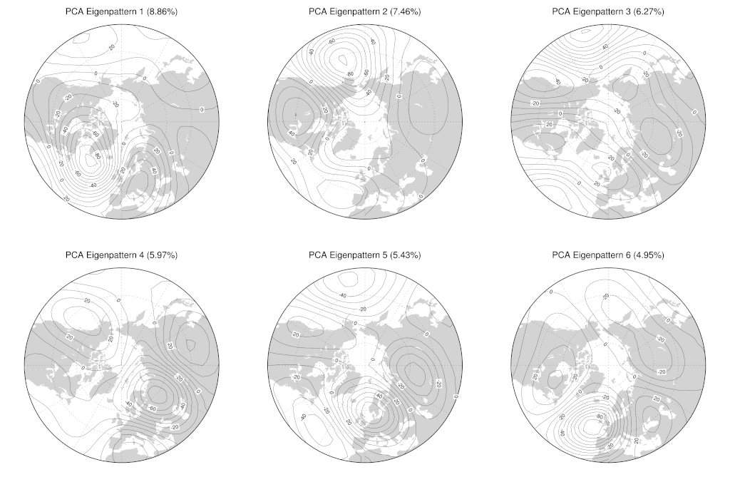
Here are the first six PCA eigenpatterns for the anomaly data (you can click on these images to see larger versions; the numbers in parentheses show the fraction of total anomaly variance explained by each PCA eigenpattern.):
For comparison here are the eigenpatterns for eigenpatterns :
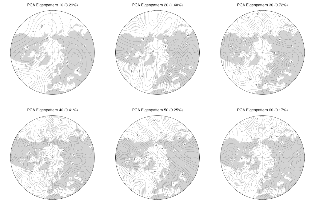
The first thing to note about these figures is that the spatial scales of variation for the PCA eigenpatterns corresponding to smaller eigenvalues (i.e. smaller explained variance fractions) are also smaller — for the most extreme case, compare the dipolar circumpolar spatial pattern for the first eigenpattern (first plot in the first group of plots) to the fine-scale spatial features for the 60th eigenpattern (last plot in the second group). This is what we often seen when we do PCA on atmospheric data. The larger spatial scales capture most of the variability in the data so are represented by the first few eigenpatterns, while smaller scale spatial variability is represented by later eigenpatterns. Intuitively, this is probably related to the power-law scaling in the turbulent cascade of energy from large (planetary) scales to small scales (where dissipation by thermal diffusion occurs) in the atmosphere But don’t make too much of that, not in any kind of quantitative sense anyway — there’s certainly no obvious power law scaling in the explained variance of the PCA eigenpatterns as a function of eigenvalue index, unless you look at the data with very power law tinted spectacles! I’m planning to look at another paper at some point in the future that will serve as a good vehicle for exploring this question of when and where we can see power law behaviour in observational data. }.
The next thing we can look at, at least in the first few patterns in the first group of plots, are some of the actual patterns of variability these things represent. The first PCA eigenpattern, for example, represents a dipole in anomaly variability with poles in the North Atlantic just south of Greenland and over mainland western Europe. If you look back at the blocking anomaly plots in an earlier post, you can kind of convince yourself that this first PCA eigenpattern looks a little like some instances of a blocking pattern over the North Atlantic. Similarly, the second PCA eigenpattern is mostly a dipole between the North Pacific and North America (with some weaker associated variability over the Atlantic, so we might expect this somehow to be related to blocking episodes in the Pacific sector.
This is all necessarily a bit vague, because these patterns represent only part of the variability in the data, with each individual pattern representing only a quite small fraction of the variability (8.86% for the first eigenpattern, 7.46% for the second, 6.27% for the third). At any particular point in time, the pattern of anomalies in the atmosphere will be made up of contributions from these patterns plus many others. What we hope though is that we can tease out some interesting characteristics of the atmospheric flow by considering just a subset of these PCA eigenpatterns. Sometimes this is really easy and obvious — if you perform PCA and find that there are two leading eigenpatterns that explain 80% of the variance in your data, then you can quite straightforwardly press ahead with analysing only those two patterns of variability, safe in the knowledge that you’re capturing most of what’s going on in your data. In our case, we’re going to try to get some sense of what’s going on by looking at only the first three PCA eigenpatterns (we’ll see why three in the next article). The first three eigenpatterns explain only 22.59% of the total variance in our anomaly data, so this isn’t obviously a smart thing to do. It does turn out to work and to be quite educational though!
The last component of the output from the PCA procedure is the time series of PCA projected component values. Here we have one time series (of 9966 days) for each of the 1080 PCA eigenpatterns that we produced. At each time step, the actual anomaly field can be recovered by adding up all the PCA eigenpatterns, each weighted by the corresponding projected component. You can look at plots of these time series, but they’re not in themselves all that enlightening. I’ll say some more about them in the next article, where we need to think about the autocorrelation properties of these time series.
(As a side note, I’d comment that the PCA eigenpatterns shown above match up pretty well with those in Crommelin’s paper, which is reassuring. The approach we’re taking here, of duplicating the analysis done in an existing paper, is actually a very good way to go about developing new data analyis code — you can see quite quickly if you screw things up as you’re going along by comparing your results with what’s in the paper. Since I’m just making up all the Haskell stuff here as I go along, this is pretty handy!)