Non-diffusive atmospheric flow #14: Markov matrix calculations
This is going to be the last substantive post of this series (which is probably as much of a relief to you as it is to me…). In this article, we’re going to look at phase space partitioning for our dimension-reduced PCA data and we’re going to calculate Markov transition matrices for our partitions to try to pick out consistent non-diffusive transitions in atmospheric flow regimes.
Phase space partitioning
We need to divide the phase space we’re working in (the unit sphere parameterised by and ) into a partition of equal sized components, to which we’ll assign each data point. We’ll produce partitions by dividing the unit sphere into bands in the direction, then splitting those bands in the direction as required. The following figures show the four partitions we’re going to use here I was originally planning to do some more work to demonstrate the independence of the results we’re going to get to the choice of partition in a more sophisticated way, but my notes are up to about 80 pages already, so I think these simpler fixed partition Markov matrix calculations will be the last thing I do on this! :

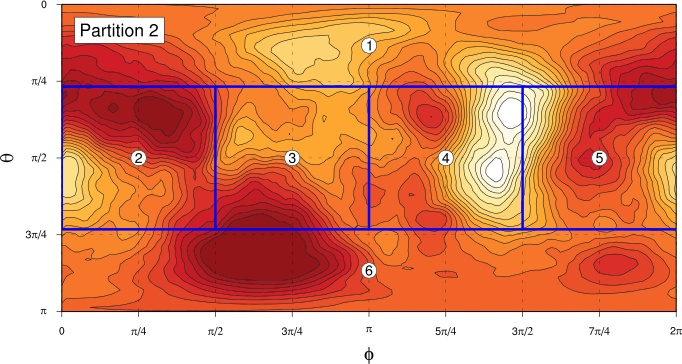


In each case, the “compartments” of the partition are each of the same area on the unit sphere. For Partitions 1 and 2, we find the angle of the boundary of the “polar” components by solving the equation
where C is the number of components in the partition. For partition 1, with N=4, this gives and for partition 2, with N=6, .
Assigning points in our time series on the unit sphere to partitions is then done by this code (as usual, the code is in a Gist):
-- Partition component: theta range, phi range.
data Component = C { thmin :: Double, thmax :: Double
                   , phmin :: Double, phmax :: Double
                   } deriving Show

-- A partition is a list of components that cover the unit sphere.
type Partition = [Component]

-- Angle for 1-4-1 partition.
th4 :: Double
th4 = acos $ 2.0 / 3.0

-- Partitions.
partitions :: [Partition]
partitions = [ [ C 0        (pi/3)   0  (2*pi)
               , C (pi/3)   (2*pi/3) 0  pi
               , C (pi/3)   (2*pi/3) pi (2*pi)
               , C (2*pi/3) pi       0  (2*pi) ]
             , [ C 0        th4      0        (2*pi)
               , C th4      (pi-th4) 0        (pi/2)
               , C th4      (pi-th4) (pi/2)   pi
               , C th4      (pi-th4) pi       (3*pi/2)
               , C th4      (pi-th4) (3*pi/2) (2*pi)
               , C (pi-th4) pi       0        (2*pi) ]
             , [ C 0      (pi/2) 0  pi
               , C 0      (pi/2) pi (2*pi)
               , C (pi/2) pi     0  pi
               , C (pi/2) pi     pi (2*pi) ]
             , [ C 0      (pi/2) (pi/4)   (5*pi/4)
               , C 0      (pi/2) (5*pi/4) (pi/4)
               , C (pi/2) pi     (pi/4)   (5*pi/4)
               , C (pi/2) pi     (5*pi/4) (pi/4) ] ]

npartitions :: Int
npartitions = length partitions

-- Convert list of (theta, phi) coordinates to partition component
-- numbers for a given partition.
convert :: Partition -> [(Double, Double)] -> [Int]
convert part pts = map (convOne part) pts
  where convOne comps (th, ph) = 1 + length (takeWhile not $ map isin comps)
          where isin (C thmin thmax ph1 ph2) =
                  if ph1 < ph2
                  then th >= thmin && th < thmax && ph >= ph1 && ph < ph2
                  else th >= thmin && th < thmax && (ph >= ph1 || ph < ph2)
The only thing we need to be careful about is dealing with partitions that extend across the zero of .
What we’re doing here is really another kind of dimensionality reduction. We’ve gone from our original spatial maps of to a continuous reduced dimensionality representation via PCA, truncation of the PCA basis and projection to the unit sphere, and we’re now reducing further to a discrete representation — each map in our original time series data is represented by a single integer label giving the partition component in which it lies.
We can now use this discrete data to construct empirical Markov transition matrices.
Markov matrix calculations
Once we’ve generated the partition time series described in the previous section, calculating the empirical Markov transition matrices is fairly straightforward. We need to be careful to avoid counting transitions from the end of one winter to the beginning of the next, but apart from that little wrinkle, it’s just a matter of counting how many times there’s a transition from partition component j to partition component i, which we call . We also need to make sure that we consider the same number, , of points from each of the partition components. The listing below shows the function we use to do this — the \texttt{transMatrix} function takes as arguments the size of the partition and the time series of partition components as a vector, and returns the transition count matrix and , the number of points in each partition used to calculate the transitions:
transMatrix :: Int -> SV.Vector Int -> (M, Int)
transMatrix n pm = (accum (konst 0.0 (n, n)) (+) $ zip steps (repeat 1.0), ns)
  where allSteps = [((pm SV.! (i + 1)) - 1, (pm SV.! i) - 1) |
                    i <- [0..SV.length pm - 2], (i + 1) `mod` 21 /= 0]
        steps0 = map (\k -> filter (\(i, j) -> i == k) allSteps) [0..n-1]
        ns = minimum $ map length steps0
        steps = concat $ map (take ns) steps0
Once we have , the Markov matrix is calculated as and the symmetric and asymmetric components of are calculated in the obvious way:
splitMarkovMatrix :: M -> (M, M)
splitMarkovMatrix mm = (a, s)
  where s = scale 0.5 $ mm + tr mm
        a = scale 0.5 $ mm - tr mm
We can then calculate the matrix that recovers the non-diffusive part of the system dynamics. One thing we need to consider is the statistical significance of the resulting components in the matrix: these components need to be sufficiently large compared to the “natural” variation due to the diffusive dynamics in the system for us to consider them not to have occurred by chance. The statistical significance calculations aren’t complicated, but I’ll just present the results here without going into the details (you can either just figure out what’s going on directly from the code or you can read about it in Crommelin (2004)).
Let’s look at the results for the four partitions we showed earlier. In each case, we’ll show the Markov transition count matrix and the “non-diffusive dynamics” matrix. We’ll annotate the entries in this matrix to show their statistical significance: , , , , , .
For partition #1, we find:
For partition #2:
For partition #3:
And for partition #4:
So, what conclusions can we draw from these results? First, the results we get here are rather different from those in Crommelin’s paper. This isn’t all that surprising — as we’ve followed along with the analysis in the paper, our results have become more and more different, mostly because the later parts of the analysis are more dependent on smaller details in the data, and we’re using a longer time series of data than Crommelin did. The plots below represent that contents of the matrices for each partition in a graphical form that makes it easier to see what’s going on. In these figures, the thickness and darkness of the arrows show the statistical significance of the transitions.
We’re only going to be able to draw relatively weak conclusions from these results. Let’s take a look at the apparent dynamics for partitions #1 and #2 shown above. In both cases, there is a highly significant flow from the right hand side of the plot to the left, presumably mostly representing transitions from the higher probability density regions on the right (around , ) to those on the left (around , ). In addition, there are less significant flows from the upper hemisphere of the unit sphere to the lower, more significant for partition #2 than for #1, with the flow apparently preferentially going via partition component number 4 for partition #2. Looking back at the “all data” spherical PDF with some labelled bumps, we see that the flow from the right hand side of the PDF to the left is probably something like a transition from bump 4 (more like a blocking pattern) to bump 2 (more like a normal flow).
I’ll freely admit that this isn’t terrible convincing, and for partitions #3 and #4, the situation is less clear.
For me, one of the lessons to take away from this is that even though we started with quite a lot of data (daily maps for 66 years), the progressive steps of dimensionality reduction that we’ve used to try to elucidate what’s going on in the data result in less and less data on which we do the later steps of our analysis, making it more and more difficult to get statistically significant (or even superficially convincing) results. It’s certainly not the case that the results in Crommelin (2004) are just a statistical accident — there really is observed persistence of atmospheric flow patterns and pretty clear evidence that there are consistent transitions between different flow regimes. It’s just that those might be quite hard to see via this kind of analysis. Why the results that we see here are less consistent than those in Crommelin’s analysis is hard to determine. Perhaps it’s just because we have more data and there was more variability in climate in the additional later part of the time series. Or I might have made a mistake somewhere along the way!
It’s difficult to tell, but if I was doing this analysis “for real”, rather than just as an exercise to play with data analysis in Haskell, I’d probably do two additional things:
Use a truncated version of the data set to attempt to the replicate the results from Crommelin (2004) as closely as possible. This would give better confidence that I’ve not made a mistake.
Randomly generate partitions of the unit sphere for calculating the Markov transition matrices and use some sort of bootstrapping to get a better idea of how robust the “significant” transitions really are. (Generating random partitions of the sphere would be kind of interesting — I’d probably sample a bunch of random points uniformly on the sphere, then use some kind of spring-based relaxation to spread the points out and use the Voronoi polygons around the relaxed points as the components of the partition.)
However, I think that that’s quite enough about atmospheric flow regimes for now…